Guitar speaker cab with a Kevlar cone speaker

Skytronic: 5 1/4'' Kevlar cone speaker

I've build a simple cab for a cheap Skytronic Kevlar cone speaker

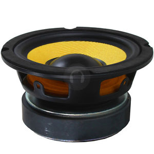Skytronic: 5 1/4'' Kevlar cone speaker

Although it sounded ok, a bit of math would benefit the sound that it produces. Note that this is not a typical guitar speaker. In what follows I will try to convince you that regular speakers (namely woofers) can be used to make great guitar cabs!

The specs for this speaker are these.

Item No.	902.420
Re	7
Le	?
Fs	55
Qms	5
Qes	.44
Qts	.41
Sd(cm2)	81
Vas(L)	5.6
Cms(uM/N)	605
Mms(g)	14.5
B x L	8.7
SPL_1W/1m2	84.8
Prms(W)	100
Pmax(W)	200
Xmax	3.5

The quantity that really one should look, because I'm doing a synthesis, is total Q; this value is a combination of the properties of the speaker taken conjointly with the cab.

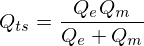
The best reference to learn how to design speaker enclosures is still the papers by Richard H. Small and Neville Thiele. So the relevant equations are the electrical Q (taken into account the output impedance of the amplifier $latex2png equation$ , $latex2png equation$ the total Qts, combines Qe and Qms, like two resistors in parallel $latex2png equation$ and the volume of the enclosure 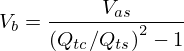$latex2png equation$ where $latex2png equation$ is the total Q of the enclosure and speaker system.

The predicted Fc frequency of the system is then $latex2png equation$

The design process can be simplified by using a dimensionless parameter $latex2png equation$ called the system compliance ratio, that can be written as $latex2png equation$

A simple GNU/Octave script will allow us to get a more clear view about the choices we are about to make.

#1;
Rg=8;

Re=7;
Fs=55
Qms=5
Qes=.44
Qts=.41;
Sd=81;
Vas=5.6;
Cms=605;
Mms=14.5;
BxL=8.7;

Qe=Qes*(Rg+Re)/Re
Qts=1./(1./Qe + 1/Qms)
eta=4*pi^2/344^3*Fs^3*Vas/Qes*1e-3

alpha=[1:.01:4];
Qtc=Qts*(1+alpha).^.5;
Vb=Vas./alpha;
Fc=Fs*(1+alpha).^.5;

clf
subplot(3,1,1)
plot(alpha,Fc,'r')
ylabel('F (Hz)')
grid
title(sprintf('Rg = %i',Rg))

subplot(3,1,2)
plot(alpha,Qtc,'r')
ylabel('Qtc')
grid

subplot(3,1,3)
plot(alpha,Vb,'r')
ylabel('Vb (l)')
xlabel('alpha')
grid

Before choosing the dimensions of the enclosure let us look at some graphs.

The next figure shows the values of Fc, Qtc and Vb as a function of alpha.

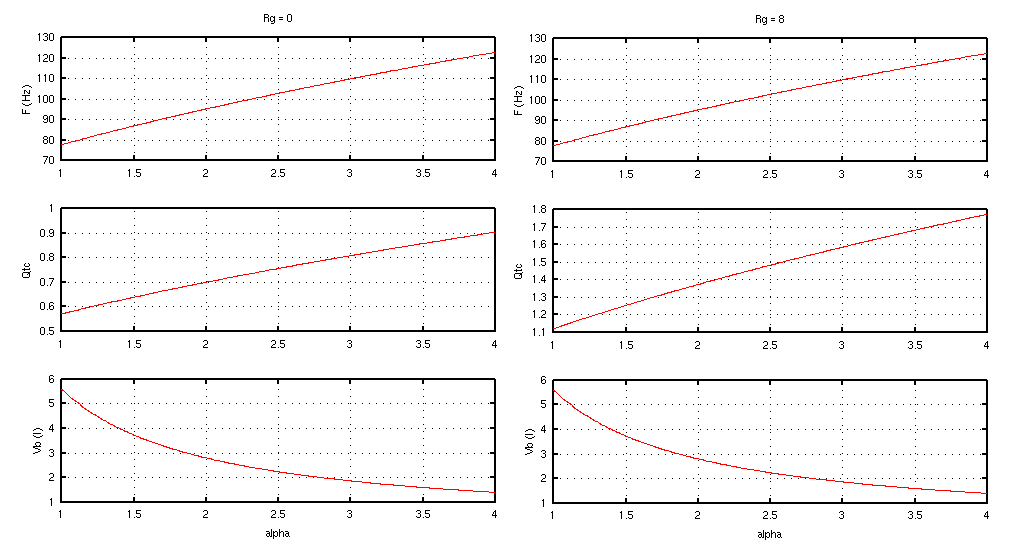Left:Amplifier output impedance Rg=0, high damping factor (infinite).Right: Amplifier output impedance Rg=8, damping factor equals 1.

The next plot shows the frequency response of a typical high damping output amplifier (not for this particular speaker).

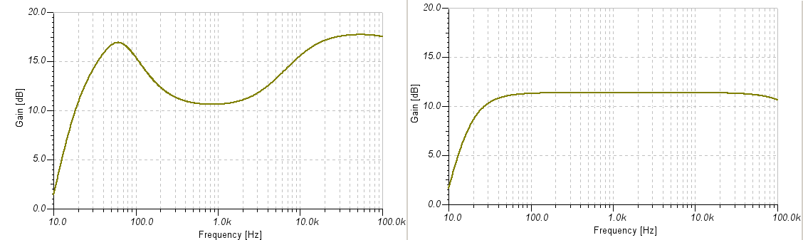Left plot: Rg=8. Right plot: Rg=0.

We see that a non-null output impedance permits the speaker to shine through, and also gives us a clear separation of bass and treble regions. This feature somewhat tames the distortion and gives the a good spectrum that we all like in guitar amplifiers (that can be found in tube/valve guitar amplifiers). This fact is one of the main reasons that a typical solid state hi-fi amplifier is found to sound terrible when fed with a distorted guitar signal.

So I'm aiming at a Rg=8 amplifier and a Fc around 80Hz (low E string), this gives $latex2png equation$ and $latex2png equation$ for $latex2png equation$ which will give a warm and dark tone (for smaller Qtc the Fc will be smaller and although it gives a clearer tone, due to the low Fs of this speaker, the final tone would be somewhat a bit mushy).

(to be continued)

Palavras chave/keywords: DIY, guitar, speaker, kevlar

Criado/Created: NaN

Última actualização/Last updated: 10-10-2022 [14:26]

Voltar à página inicial.